This project aimed to recommend movies that would be a good match for the user’s preferences and would be suitable for each person individually. We needed this system because there were numerous fantastic contents in our platform that the user might not have come across. But if they become aware of them, they could discover items they really enjoy.

In this project, I used a hybrid model which combined two common approaches: Content-based Filtering and Collaborative Filtering.

Content-based Filtering

As its name implies, the content-based filtering approach recommends new movies which are similar to the content users have engaged with. To measure the similarity between these movies, we created a matrix item-attribute for all the films available in our platform, then calculated the cosine similarity for each pair of item vectors. Then, for each user, the recommended items will be those with the highest similarity scores to the movies they’ve watched, and also have never been shown to this user before.

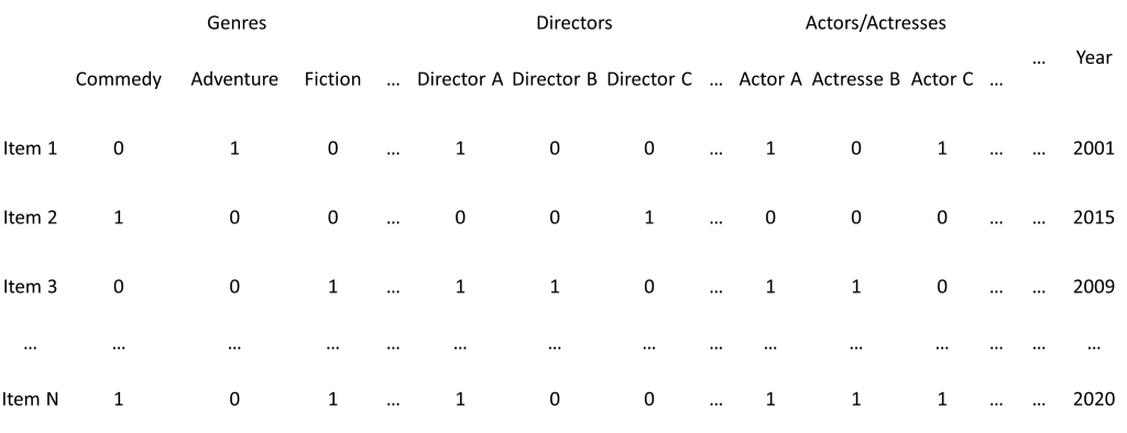
Item-Feature matrix

In this matrix, each row is a vector of a movie constructed from several features such as film production company, movie’s genre, producer, director, actors/actresses, year published, movie duration, and so on.

Singular Value Decomposition (SVD)

Since there were thousands of directors, actors, actresses and other categorical features, creating dummy variables for these features generated very long row vectors in the item-feature matrix. We used SVD technique to reduce the length of these vectors in order to speed up the cosine similarity calculations for item pairs.

So, what is SVD and why is it used for reducing the dimensionality of the data? The three points of view below will explain it.

• First, it’s a method for transforming correlated variables into a set of uncorrelated variables. This transformation better reveals various relationships among the original data items.
• Second, it’s a method for identifying and ordering the dimensions along which data points exhibit the most variation.
• Third, identifying where the most variation is allows us to find the best approximation of the original data points using fewer dimensions. For example, both figures below display the transformation of 2D data into 1D data. The better transformation is the figure on the right as the red line in this figure captures more variation (more information) in the original data.

Mathematically, SVD decomposes the matrix A as:

Anm = UnnSnmVTmm

where: UTU = I, VTV = I.
Unn and VTmm are orthonormal matrices whose columns and rows are orthonormal vectors;
Smn is a diagonal matrix, can be non-square, but only the entries on the diagonal could be non-zero.

Before decomposing a matrix using SVD, we need to know about eigenvalues and eigenvectors. Intuitively, eigenvalues determine how much the space is scaled along specific directions, while eigenvectors specify these directions. For a matrix W, then a nonzero vector v is the eigenvector of W if: 
Wv = λv
Then the scalar λ is called an eigenvalue of W, and v is said to be an eigenvector of W corresponding to λ.

Calculating the SVD consists of finding the eigenvalues and eigenvectors of AAT and ATA since:
- The orthonormal eigenvectors of AAT make up the columns of U,
- The orthonormal eigenvectors of ATA make up the columns of V,
- S is a diagonal matrix containing the square roots of eigenvalues from from AAT or ATA in descending order (AAT and ATA have the same set of eigenvalues even that they can have different size).

In Recommendation System, we used a truncated SVD to decompose the item-feature matrix as below:

A_nm = U_nxrS_rxrV^T_mxm

where S is a rxr square diagonal matrix, with r being the rank of A. The rank of a matrix refers to the maximum number of linearly independent rows or columns in the matrix, which tells us how many unique directions or dimensions that its rows or columns span. The figure below demonstrates the truncated SVD decomposition for the item-feature matrix.

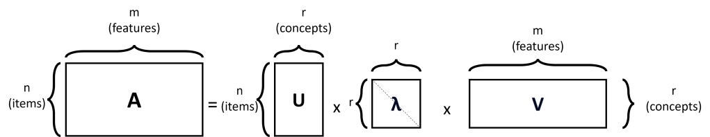
Then, we used the matrix U, which captures the latent characteristics of the items in the original dataset, to calculate the cosine similarity for its row vectors.

Cosine similarity

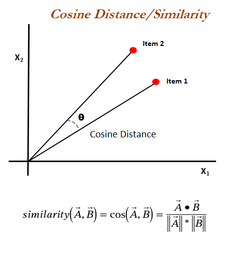
We measured the similarity of the movies by converting these movies to vectors and calculated their cosine similarity. This metric calculates the cosine of the angle between the vectors, which reflects how closely they align with each other.

Recommendation

For each user, we calculated the cosine similarity of the movies available in our system with the user’s preferences and recommend the top-N movies with the highest similarity to this user.

Collaborative Filtering

Collaborative Filtering approach centers around the idea that users with similar past preferences tend to have similar future preferences. It starts by constructing a user-item interaction matrix, representing user interactions. This approach has two main sub-branches: Neighborhood-Based and Latent Factor Models. While both use past interactions for predictions, Latent Factor Models uncover hidden factors that contribute to the observed interactions, instead of directly calculating similarities like in Neighborhood-Based methods.

Due to the nature of user interactions, the user-item interaction matrix often contains gaps because not all users have interacted with all items. Now, the challenge is to predict how a user might rate an item they haven’t yet interacted with. This is where latent factor models come into play.

User-Item Matrix

Latent Factor Models and Matrix Factorization

Matrix factorization is built on the assumption that there exists a latent (hidden) feature space that drives user preferences and item characteristics. By breaking down the original matrix into user and item latent vectors, matrix factorization deciphers these latent features. Such that, it uses these learned latent factors to estimate missing ratings, filling in the gaps and enabling accurate recommendations. The figure below illustrates the factorization.

The matrix factorization can also be expressed through a mathematical formulation as follows:

r_ui ≈ q_i^Tp_u

where r_ui is user u’s rating of item i, p_u is latent vector of user u, and q_i is latent vector of item i. The objective function is typically formulated as the sum of squared errors with regularization on the set of known ratings:

Finding p and q that minimizes this objective function can be done using optimization techniques like Stochastic Gradient Descent (SGD) or Alternating Least Squares (ALS). Here are the learning steps:

To minimize the objective function using SGD, we update the latent factor matrices p and q iteratively based on the gradient of the error with respect to p and q for each observed user-item interaction. In ALS, we alternate between updating the user latent factors and the item latent factors while keeping the other fixed.

Prediction and Recommendation

After finding matrix p and q, we can calculate the predicted ratings for movies the user has not yet interacted with. The predicted rating is obtained by q_i^Tp_u. For each user, rank the movies based on their predicted ratings. Recommend the top-N movies with the highest predicted ratings to the user.

Hybrid model

Since Content-based Filtering and Collaborative Filtering have their own strengths and weaknesses, combining them can provide more accurate recommendations by compensating for the limitations such as lack of serendipity and cold-start problem.

Discussion

Besides the algorithms, when built this Recommendation System, we had to consider many aspects such as real time recommendations, big data and scalability, evaluation metrics, implicit and explicit data, and so on.

If you don’t want to start from scratch, you can find some templates for Recommendation System provided by PredictionIO to start. These templates are like a starting point that you can grab and tweak to match your specific needs.

References

• Y. Koren, R. Bell and C. Volinsky, “Matrix Factorization Techniques for Recommender Systems,” in Computer, vol. 42, no. 8, pp. 30-37, Aug. 2009, doi: 10.1109/MC.2009.263.
• Baker, Kirk. “Singular Value Decomposition Tutorial.” The Ohio State University, 29 Mar. 2005, vol. 24, pp. 22.
• Cosine Similarity Illustration. In “Statistics for Machine Learning” by P. Dangeti, O’Reilly, URL: https://www.oreilly.com/library/view/statistics-for-machine/9781788295758/eb9cd609-e44a-40a2-9c3a-f16fc4f5289a.xhtml