Customer churn prediction was a year-long project in which I was deeply involved. This project was not only deployed but also published in the 2017 IEEE International Conference on Big Data. For comprehensive details on this work, feel free to explore our publication.
Do, Duyen, Phuc Huynh, Phuong Vo, and Tu Vu. “Customer churn prediction in an internet service provider.” In 2017 IEEE International Conference on Big Data (Big Data), pp. 3928-3933. IEEE, 2017.
https://doi.org/10.1109/BigData.2017.8258400
Achievement
When we compared it to the earlier basic approach by the customer service team, using machine learning to predict churn customers works much better. The precision went up by almost 30%, from 15% to 45.71%. This means the company can save time, money, and effort. Additionally, the model identified many customers facing service issues, allowing the customer service department to help them effectively and promptly.
The problem
You may already know the importance of customer retention. Customers are crucial for sustaining business growth and profitability. Losing customers is not only about losing profits; it can also pose a threat to a company’s very foundation in the face of their competitors. In reality, providing customer care demands significant time, effort, and resources. To enhance this process, the Customer Churn Prediction project was initiated to predict customers who are likely to leave the services. This allows the customer service department to prioritize customers, focus on those requiring immediate attention, such that they can then proactively ensure timely care and effective retention.
The Challenge: Imbalanced Data in Churn Prediction
For our problem, we categorized it as a binary classification predictive modeling task with two classes: churn and non-churn. The main challenge lies in imbalanced data. As you’re aware, the lower the churn rate, the more favorable it is for business and the more challenging it becomes for predictive models. In our case, churners represent 2%, with non-churners comprising 98% of the dataset.
Feature Engineering: Extracting the Essence
This phase was both exhilarating and optimistic, as we dived into data analysis to gain deeper insights into customer issues. During this step, we collaborated with the other departments to deeply understand business operations and policies, gathering and understanding the data they provided. Our goal was to identify impactful features for churn prediction. Interestingly, even though some features might not have been used in the models, they provided valuable insights for improving service quality.
This step consumed a lot of time as we analyzed any types of data that were available. These data can be grouped into three types:
- Customer information: registration and termination dates, location, service and cable types, bandwidth, payment history, promotions, and more.
- Customer usage data in telecommunications: connection between user’s devices and the company’s server (initiation and disconnection times, rejection reasons, device types, etc.) and daily usage (download and upload volume).
- Customer service records: inbound and outbound call histories, satisfaction surveys, maintenance and support logs, etc.
In additional, we also generated a significant number of new features from the existing data, assessed their seasonal impact (e.g., Tet holiday). Since there were too many features, conducting statistical methods for all of them was inefficient. Instead, we used several techniques like mRMR, Random Forest, Brute-force, Top-down, and Bottom-up approaches to rank feature importance. And the winner for feature importance ranking is XGBoost. Below are visualizations for some of the most important features.
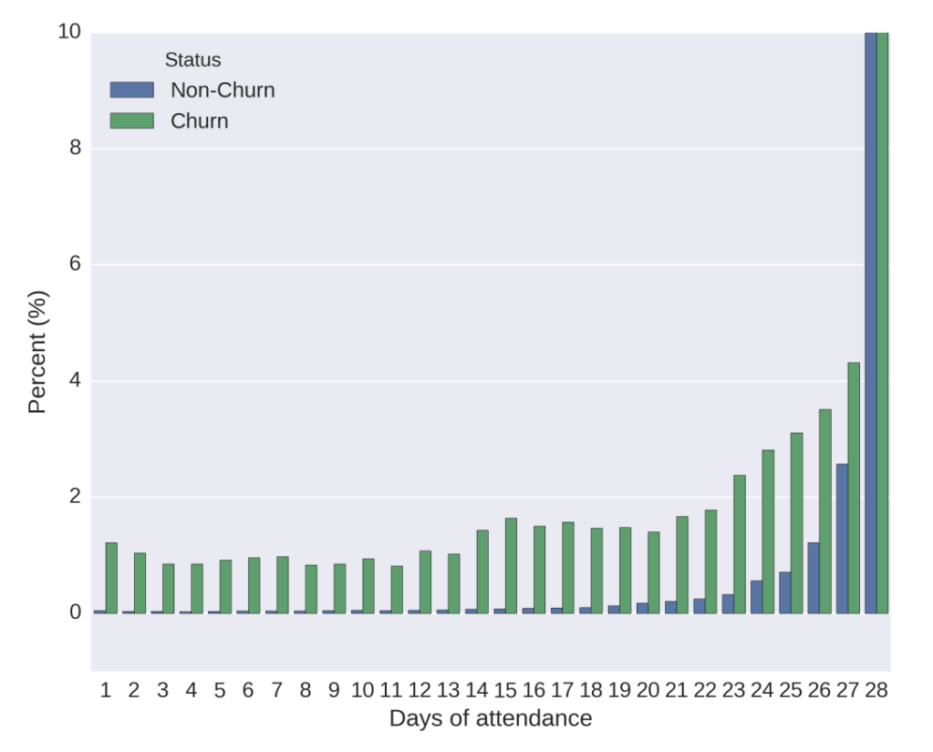

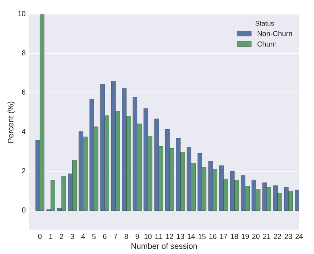
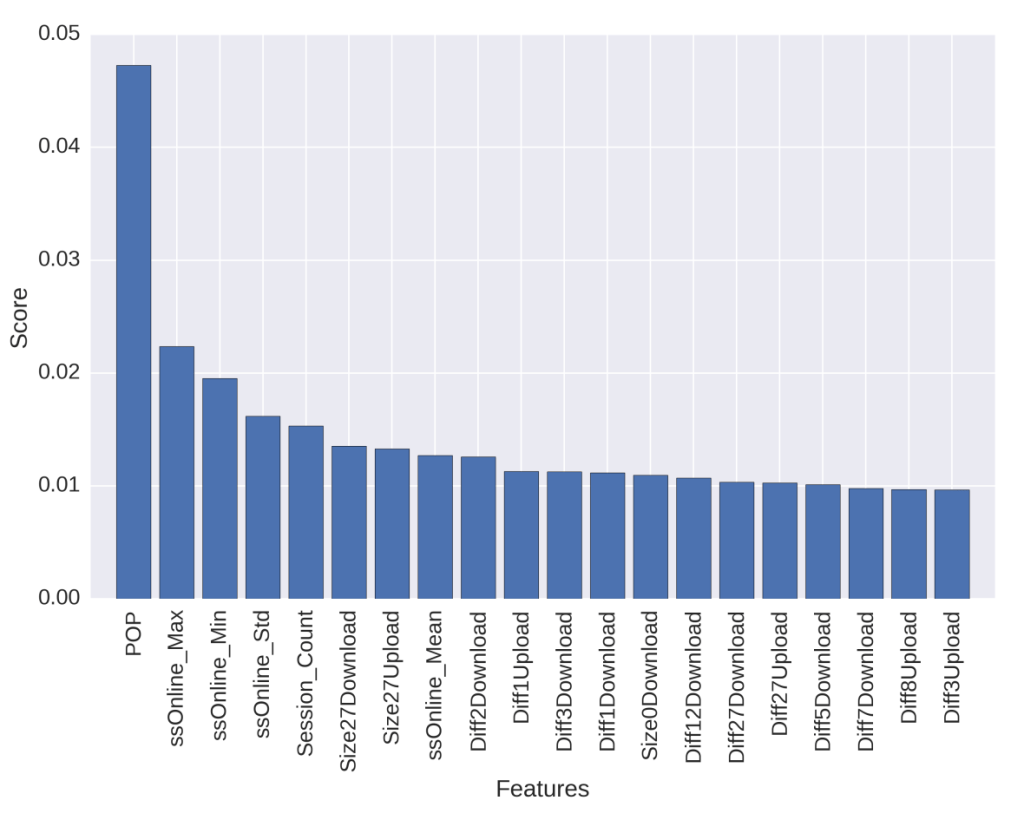
The best features selected by the XGBoost feature important ranking approach include:
- Point of Present (POP): local access points of the ISP
- Session features (max, min, count, …)
- Download and upload features (daily size, difference between two consecutive days, etc.)
- Service types
- And more.
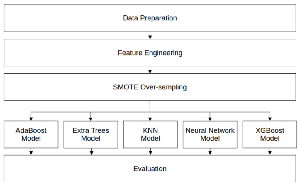
Balancing the classes: Tackling Imbalanced Data
This is also an important task that has a significant impact on the performance of the models. In this step, we tried both under-sampling approach such as Random Undersampling, Cluster Centroids, Tomek Links, Edited Nearest Neighbors (ENN),… and over-sampling approach like Random Oversampling, SMOTE, ADASYN,… The final technique we chose for balancing the classes was SMOTE (Synthetic Minority Oversampling TEchnique) which generates synthetic instances by interpolating between existing minority class instances, effectively creating new data points.
The Model Face-Off: Predictive Modeling and Evaluation
We were eager for this step, filled with excitement to wait for the outcome of the models.
Classification Metrics
As we’ve defined our problem as a classification predictive modeling task with extremely imbalanced binary classes, we evaluated the model’s performance by considering both precision and recall. To balance these metrics, we used the F1-score. Additionally, in this context, the positive class will correspond to churners, as they are our target for prediction.
Precision = TP / Predicted positive = TP / (TP + FP)

Recall = TP / Real positive = TP / (TP + FN)

F1-score: a trade-off with equal weight given to both precision and recall
F1-score = (1 + β2) * (Precision * Recall) / (β2*Precision + Recall) where β=1
Predictive Modeling
Several predictive models enter the arena: AdaBoost, Extra Trees, k-Nearest Neighbors (k-NN), Neural Network, and XGBoost.
Outputs and Threshold?
These models are put through their paces, each with its own set of parameters fine-tuned using GridSearchCV and measured by F1-score to achieve optimal performance.
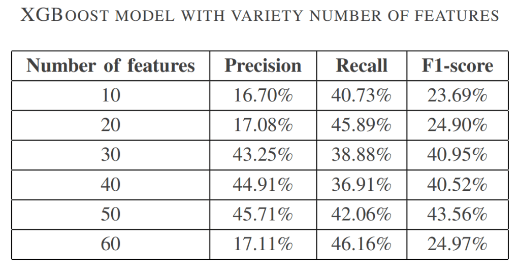
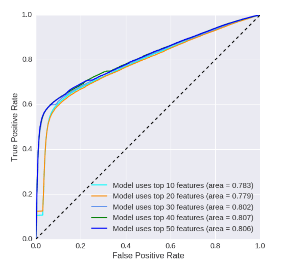
Based on the XGBoost feature importance scores, we experimented with varying numbers of top-ranked variables to identify the optimal model-feature alignment before comparing the models’ performance.
Beside is an example for the XGBoost model with different numbers of features. The Table and ROC curves illustrate how the number of features impacts its performance.
And the Winner is…
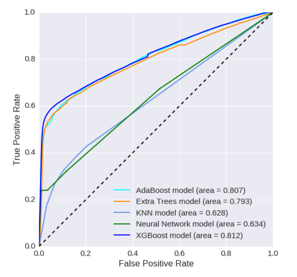
Out of all the models, XGBoost stands out as the top performer. It accurately spots possible churners with 45.71% precision and 42.06% recall. Apart from accuracy, we also looked into the time and resources used for these models. The experiments demonstrated that the differences were insignificant. The performance of these models illustrated in the upcoming figures.
| No. | Model | Precision | Recall | F1-score |
| 1 | XGBoost | 45.71% | 42.06% | 43.56% |
| 2 | Extra trees | 35.57% | 42.98% | 38.92% |
| 3 | AdaBoost | 25.12% | 51.39% | 33.74% |
| 5 | Neural Networks | 32.24% | 23.98% | 27.50% |
| 4 | k-NN | 6.06% | 32.75% | 10.22% |
The performance of models
Conclusion
Applying machine learning for churn prediction significantly outperformed the previous basic approach, boosting precision from 15% to 45.71%. This enhances efficiency and enables timely assistance to customers with service problems.
In a bigger picture, what we did can be used for other similar classification tasks where data is imbalanced.

Leave a comment